Closed Models Are Just Someone Else's Tokens

In my last post, we took our first steps building with LLMs by calling closed models behind proprietary APIs. Closed models, though, run in someone else's cloud. That may be a dealbreaker if you need more control and data privacy.

Closed models currently lead in terms of ability, but I believe that in the long term, open models will likely prevail, much as Linux eventually surpassed proprietary Unix in the server market. Always bet on open source, given enough time.

Until then, open-weight models are already practical and worth exploring for production if your use case recommends it.

People often refer to "open source models," but that term can be misleading. For example, the Llama models provide weights anyone can download and run, but they don't disclose their training data or all the code used to build them.

In other words, these models are open-weight, but not fully open-source. The level of openness varies between labs and models, but practically speaking, you can deploy, fine-tune, and serve any open-weight model yourself.

To deploy a model, you'll need three things:

1. Model weights
2. An inference server
3. Hardware to run it

In this post, you'll learn how to select the right open-weight model, navigate licensing requirements, handle context-window limitations, choose an inference server, determine hardware needs, and plan deployment architectures for running your own models in production.

Choosing a model

Not all models are created equal. Open-weight models come in a range of sizes and capabilities. Smaller models will run on consumer hardware and generally provide fast inference at lower operational costs, but their answers will often lack the breadth and nuance of the largest models. Generally speaking, larger models tend to provide better reasoning ability, fluency, and general knowledge at the expense of compute costs.

Parameter count is not a perfect proxy for quality, though. It's worth noting that recent efficiency gains now enable some smaller models to punch above their weight. Qwen 3 4B, for example, matches the performance of the earlier Qwen 2.5 72B with eighteen times fewer parameters. Larger models still tend to have the highest absolute capability, but these efficiency improvements mean you should weigh both size and quality when selecting a model.

You'll want to select a model that suits both your use case and the available hardware resources. For quick experiments, small and medium models are usually sufficient. For production, you may choose larger models assuming your hardware can reliably serve them under real-world user load, or fine-tune a smaller model on your own data to strike a balance between performance and quality.

You also don't have to choose just one model. In practice, applications often employ a combination of models, each tailored to the specific needs of particular tasks. Just as you might select OpenAI's o3 reasoning model for complex coding or math problems and something lighter like GPT-4o mini for simpler tasks like parsing text with structured outputs, the same applies when working with open-weight models.

Smaller models make sense, provided they reliably meet your task requirements. If a lighter model can deliver the necessary accuracy, you'll benefit from lower compute costs, faster responses, and better GPU efficiency. For more complex tasks that require advanced logic, larger reasoning models remain preferable, despite higher inference costs.

The key insight is to match your model selection to individual tasks. It would be unusual and likely inefficient for an application to rely on just a single model. You'll need to balance speed, cost, capability, and the operational complexity of managing multiple models in production.

Licensing considerations

Selecting an open-weight model involves more than comparing capability and hardware requirements. Licenses also come into play, particularly if your use case involves commercial products, redistribution, or regulated environments.

Models such as Qwen, DeepSeek, and Mistral are typically released under permissive licenses, like Apache 2.0 and MIT. These licenses impose minimal restrictions, allowing commercial use, redistribution, fine-tuning, and deployment without any friction. Essentially, the model becomes yours to use, provided proper attribution is maintained. This is likely the best case scenario for you.

In contrast, providers like Meta and Google introduce additional restrictions via community agreements and usage policies. Meta's Llama models, for instance, include an Acceptable Use Policy that explicitly prohibits their use in military applications and other sensitive domains. If you're a defense contractor, for example, this might be a problem unless you can reach a contractual agreement.

Google's Gemma license similarly carries its own restrictions. While outputs from Gemma remain yours, any new model created by distillation or similar techniques to replicate Gemma's capabilities inherits Gemma's original licensing restrictions. Additionally, Google's terms grant them the right to terminate your license if they determine you're in violation, creating potential business continuity risks even for self-hosted deployments.

Finally, not all open-weight models permit commercial use. Salesforce's xLAM-2 models ship under CC-BY-NC-4.0, which prohibits commercial deployment. Cohere's Command-R Plus, another example, carries similar restrictions, limiting it to research and other non-commercial purposes.

Licensing deserves careful attention. If your use case demands clarity, models under permissive licenses are the safest choice. Models with community agreements may still be viable, but only after thoroughly understanding and accepting the specific obligations and risks these licenses entail.

Context window

A model's context window is the maximum length of tokens that the model can process at once, including your prompt and the generated tokens. Early models like GPT-2 and GPT-3 were limited to short contexts of a couple thousand tokens or less, roughly the length of a brief blog post. GPT-3.5 expanded the context to 16K tokens, providing sufficient space to handle a typical white paper or lengthy essay comfortably.

In late 2023, models started supporting larger context windows of up to 128K tokens. That is about the length of J.R.R. Tolkien's 320-page novel The Hobbit. More recently, some models have expanded context windows to one million tokens or beyond, long enough to hold The Hobbit, the thousand-plus pages of The Lord of the Rings, and still leave room for the model's reply.

Currently, a context length of 128k tokens is a comfortable standard among open-weight models. Even more ambitious is Llama 4, which claims support for a 10 million token context window, although the efficacy and economics of that context size remain questionable.

Just because a model accepts a million tokens doesn't mean it understands them. Previous research has shown that models, even those adapted for long contexts, often suffer a measurable drop in retrieval accuracy as context length increases.

Recent benchmarks have found that none of the seven frontier LLMs tested retained stable understanding beyond 64k tokens. Similarly, evaluations indicate that current LLMs generally struggle with length requirements and information density in long-text generation, with performance deteriorating notably as the context length increases.

Beyond comprehension, longer prompts introduce latency and compute costs. Longer inputs require more compute resources and thus take longer to process. As an illustration, I benchmarked latency in Llama 4 using the Lambda Inference API, measuring time to first token for inputs from 100 to 1 million tokens.

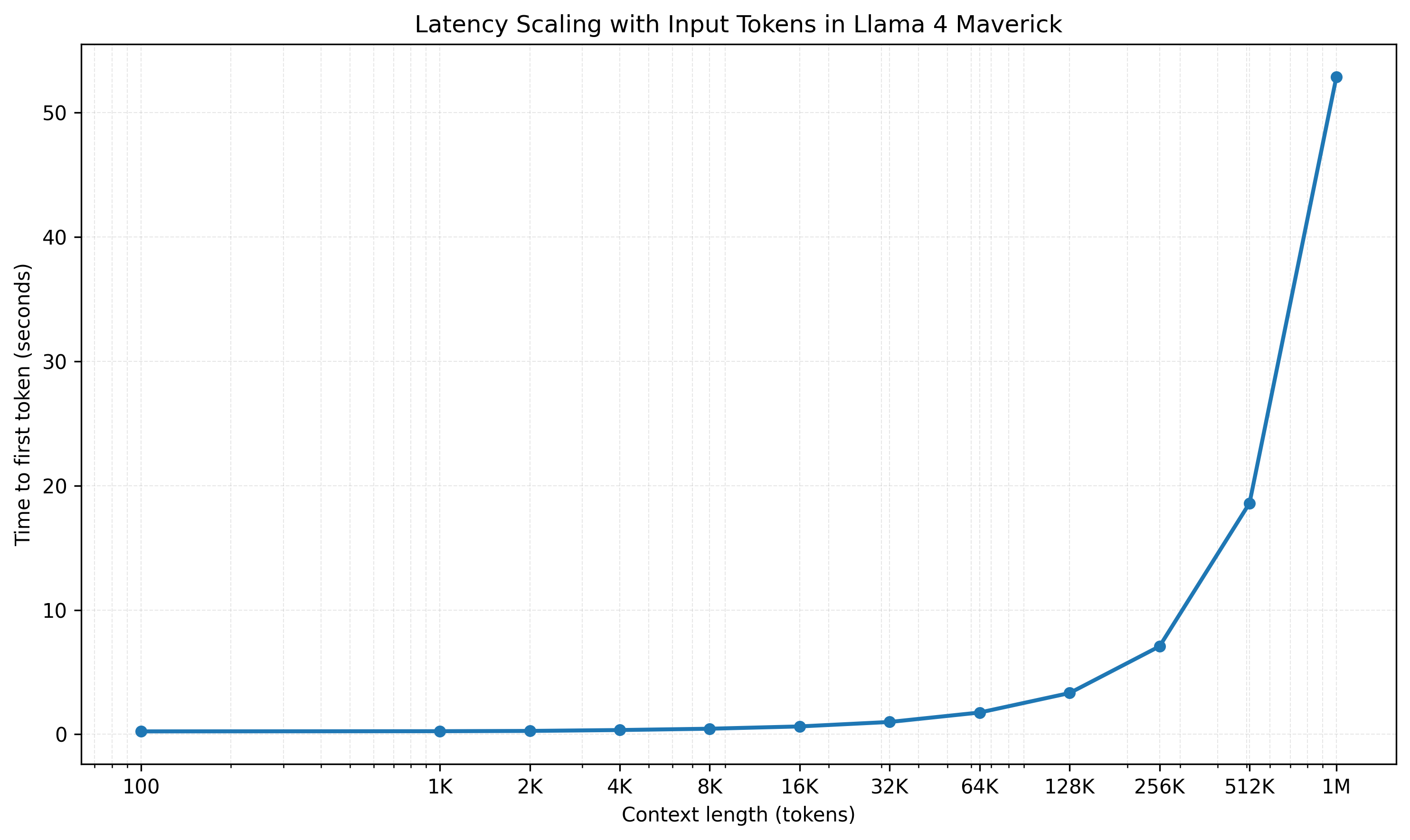
Below about 32K tokens, response times remain interactive, under one second. As context length grows toward 256K tokens, latency rises gradually to around seven seconds. Beyond this, latency sharply increases, about one minute at 1 million tokens.

Latency translates into operational costs. Even if you self-host models, more tokens mean higher compute loads and infrastructure expenses. Closed APIs bill explicitly by token count, but self-hosted systems indirectly face similar tradeoffs. Larger contexts can still make sense, but only when their benefits outweigh these costs.

Choosing an inference server

The simplest way to run inference is with an inference library such as Hugging Face Transformers. It handles model loading, tokenization, and generation in just a few lines of code:

from transformers import AutoModelForCausalLM, AutoTokenizer

model = AutoModelForCausalLM.from_pretrained("Qwen/Qwen3-4B", torch_dtype="auto", device_map="auto")
tokenizer = AutoTokenizer.from_pretrained("Qwen/Qwen3-4B")

inputs = tokenizer(["The secret to baking a good cake is "], return_tensors="pt").to("cuda")
outputs = model.generate(**inputs, max_length=30)
response = tokenizer.batch_decode(outputs)[0]

You could wrap this in a web server and call it done:

from fastapi import FastAPI

app = FastAPI()

@app.post("/generate")
async def generate(payload: dict):
    text = payload["prompt"]
    inputs = tokenizer(text, return_tensors="pt").to("cuda")
    outputs = model.generate(**inputs, max_length=30)
    return {"response": tokenizer.batch_decode(outputs)[0]}

This works, but it's not production-ready. Each request blocks the GPU until completion. Memory sits idle between requests. There's no batching, no optimization, and no proper error handling. The GPU you paid thousands of dollars for spends most of its time waiting.

Real production deployment requires an inference server that can handle concurrent users, efficiently batch data, and manage memory effectively. The server manages request queuing, dynamic batching, memory allocation, and API compatibility. Your choice here directly impacts both performance and operational complexity.

Two main options are vLLM and Text Generation Inference (TGI). Both implement continuous batching, a technique that dynamically groups requests to maximize GPU utilization. Without continuous batching, your expensive GPU sits idle between requests. With it, the hardware processes multiple requests simultaneously, significantly improving throughput.

vLLM has become a standard for many deployments. The project implements PagedAttention, which manages GPU memory like a virtual memory system. This allows vLLM to handle more concurrent requests than naive implementations would permit.

Installation is straightforward:

pip install vllm

Starting a server requires minimal configuration:

from vllm import LLM, SamplingParams

prompts = [
    "Hello, my name is",
    "The president of the United States is",
    "The capital of France is",
    "The future of AI is",
]
sampling_params = SamplingParams(temperature=0.8, top_p=0.95)

llm = LLM(model="Qwen/Qwen3-4B")

outputs = llm.generate(prompts, sampling_params)

for output in outputs:
    prompt = output.prompt
    generated_text = output.outputs[0].text
    print(f"Prompt: {prompt!r}, Generated text: {generated_text!r}")

For production, you'll typically run vLLM as an API server. The open source community has basically converged on OpenAI's API specification as the standard, which vLLM faithfully implements. This compatibility means your code works unchanged whether pointed at OpenAI or your own servers.

vllm serve Qwen/Qwen3-4B

Once running, you interact with it exactly like OpenAI's API, just pointing to your own base URL:

curl "http://localhost:8000/v1/chat/completions" \
    -H "Content-Type: application/json" \
    -d '{
        "model": "Qwen/Qwen3-4B",
        "messages": [
            {
                "role": "user",
                "content": "Write a one-sentence bedtime story about a unicorn."
            }
        ]
    }'

While the API is compatible, the implementations differ. For example, vLLM uses XGrammar or llguidance for structured outputs, open-source libraries you can inspect and modify. OpenAI's implementation remains proprietary. This transparency extends throughout the entire stack. There is no more black box.

TGI takes a different approach. It emphasizes ease of deployment and broader model support. TGI integrates tightly with the Hugging Face ecosystem, making it simple to deploy any model from their hub.

Running TGI typically involves Docker:

model=Qwen/Qwen3-4B
volume=$PWD/data

docker run --gpus all --shm-size 1g -p 8080:80 -v $volume:/data \
    ghcr.io/huggingface/text-generation-inference:latest \
    --model-id $model

Both servers implement quantization, which reduces model precision to save memory and increase speed. An 8-bit quantized model uses half the memory of its 16-bit counterpart with minimal loss in quality. This makes larger models accessible on smaller hardware budgets.

Performance differences between vLLM and TGI depend heavily on your specific workload. vLLM generally edges ahead in raw throughput benchmarks, particularly for high-concurrency scenarios. TGI often provides a better out-of-the-box experience and broader hardware compatibility.

Your choice depends on your priorities. If you require maximum performance and are willing to adjust parameters, vLLM is typically the preferred choice. If you value ease of deployment and want something that just works, TGI might be a better fit for you.

Other options exist for specific use cases. TensorRT-LLM from NVIDIA provides extreme optimization for NVIDIA hardware. SGLang optimizes structured outputs and complex workflows. vLLM and TGI will cover most general-purpose deployments.

The inference server you choose becomes part of your infrastructure. You should consider not just current performance, but also community support, update frequency, and compatibility with your existing toolchain. The best server is the one your team can operate reliably at scale.

Hardware requirements

Understanding hardware requirements starts with a simple calculation. Models require approximately 2 bytes per parameter at 16-bit precision, or around 2 GB per billion parameters. A 7 B-parameter model requires roughly 14GB of GPU memory. An 8-bit quantized version needs half that. This napkin math gets you in the ballpark, but real deployments need more nuance.

GPU memory isn't just for model weights. The KV cache stores attention states during generation, increasing in size with both batch size and sequence length. A production deployment serving multiple concurrent users may require 50-100% more memory than the base model size. Running out of GPU memory means throttling throughput or significantly degrading latency.

NVIDIA is still the default choice for ML workloads. Their CUDA ecosystem has a decade head start, and most inference software assumes NVIDIA hardware as the default option. Blackwell is their newest chip, but the H100 remains the standard in most data centers. The older A100 handles many jobs fine. For smaller models, consider the L40S, L4, or A10G for a cost-effective option.

Consumer GPUs are suitable for testing but often fail in production. The RTX 4090 and RTX 5090, for example, both cost far less than server GPUs. However, they lack error-correcting memory, fast links between GPUs, and are not designed for the continuous operation required in production. Perfect for development, risky for production.

AMD's MI300X (192GB) is breaking NVIDIA's monopoly. The massive VRAM on AMD cards enables running decent-sized models on single GPUs. However, software support lags. You'll spend time debugging issues that just work on NVIDIA. Unless you have specific reasons, NVIDIA remains the safe choice.

Your production nodes will likely have multiple GPUs, especially for serving large models. Tensor parallelism splits matrix operations across GPUs. Pipeline parallelism splits models layer by layer, typically across multiple nodes.

Efficiency measures how closely throughput scales with the number of GPUs. Tensor parallelism achieves higher efficiency, typically 85–95%, compared to pipeline parallelism, which typically ranges from 60–80%.

Choose tensor parallelism when your model fits on multiple GPUs within a single node. Otherwise, use pipeline parallelism. Tools like vLLM handle both automatically. Set --tensor-parallel-size or --pipeline-parallel-size accordingly.

Start with a single GPU deployment when possible for simplicity. Scale to multiple GPUs as memory or throughput needs grow. A 70B model requires at least two 40GB A100s or four 24GB L4s, for example. The sweet spot is often the minimum GPU count that fits your model comfortably.

Memory bandwidth matters as much as capacity. The H100's 3.35TB/s bandwidth means faster token generation than an A100's 2TB/s, even for models that fit comfortably on both. Higher bandwidth in newer GPUs directly improves performance.

CPU and system RAM requirements are modest compared to GPU demands. Any modern server CPU suffices. Plan for at least 64-256GB of system RAM to handle model loading and request buffering. Fast NVMe storage helps with model loading times but doesn't impact inference performance.

Cloud providers simplify hardware access. AWS, GCP, Azure, and specialty providers like Lambda or CoreWeave rent GPUs by the hour. This allows you to match hardware to workload without incurring capital investment. Start with on-demand instances and move to reserved pricing once you understand your usage patterns.

For on-premise deployments, consider the total cost of ownership. GPUs generate heat and consume power. An H100 draws 700W at full load. Cooling and power infrastructure can match or exceed the costs of hardware. Many teams find that cloud deployments are more cost-effective once these factors are considered.

Hardware sets hard limits on what's possible. No amount of optimization makes a 405B model fit on a 24GB GPU. Start with clear requirements, then work backwards to hardware. It is better to overspecify initially than to discover limits in production.

Deployment architectures

Production deployments typically start with a single node and one or more GPUs. As user demand grows, you may introduce redundancy, geographic distribution, and scaling techniques to support increased capacity. Begin with the simplest possible architecture, then evolve it based on your real-world load and reliability needs.

The next step might be placing a load balancer in front of multiple inference servers. Each server runs independently with its own GPU and model copy. Requests are distributed across servers based on availability. This stateless design scales horizontally and handles server failures gracefully.

# Simple load balancer configuration with nginx
upstream inference_backend {
    least_conn;
    server inference1.internal:8000;
    server inference2.internal:8000;
    server inference3.internal:8000;
}

Request routing can be more sophisticated. Different models might run on different GPU types. Route small models to less expensive GPUs, and large models to more powerful ones. Some inference servers support model routing natively. Others require external coordination.

Kubernetes has become the standard for container orchestration. It handles pod scheduling, health checks, and automatic scaling. However, GPU scheduling in Kubernetes requires configuration. The NVIDIA device plugin enables access to the GPU, but you'll need to handle node affinity to ensure that pods are assigned to GPU nodes.

Model loading time creates operational challenges. Large models take minutes to load from disk to GPU memory. During scaling events or pod restarts, users experience delays. Solutions include maintaining warm pools of pre-loaded instances or utilizing persistent volume caches to expedite loading.

For global applications, geography matters. Inference latency includes network round-trip time. A server in US-East adds 100ms+ latency for European users. Multi-region deployments require model replicas in each region, which increases costs but improves the user experience.

Some teams separate compute-intensive from memory-intensive workloads. A CPU fleet handles embedding lookups and caching. A GPU fleet processes generation requests. This hybrid approach optimizes resource utilization but increases architectural complexity.

Canary deployments and blue-green strategies work differently for ML systems. Model behavior can change subtly from one version to another. Progressive rollouts with monitoring catch issues before they impact all users. Route a percentage of traffic to new model versions, monitor quality metrics, and then gradually increase.

Batch processing presents different challenges from real-time serving. Overnight jobs can tolerate higher latency in exchange for better throughput. Configure inference servers differently for batch workloads. Increase batch sizes, relax latency constraints, and optimize for GPU utilization over response time.

State management becomes critical at scale. While individual inference requests are stateless, applications often need conversation history or user context. External state stores, such as Redis, maintain this data. The inference layer stays stateless while the application layer manages state.

Performance optimization

The gap between naive and optimized inference can be 10x or more. Understanding optimization techniques helps you serve more users with less hardware. Begin with the highest-impact optimizations before proceeding to complex tuning.

Quantization reduces numerical precision while maintaining model quality and accuracy. Most models are trained in 16-bit or 32-bit floating-point. Quantizing to 8-bit floating point (FP8) halves memory usage and increases throughput with minimal quality loss.

# Using vLLM with quantization
llm = LLM(
    model="Qwen/Qwen3-4B",
    quantization="fp8"
)

Alternative quantization methods, such as AWQ and GPTQ, compress to 4-bit integers, which is useful when memory is constrained. FP8 typically provides the best balance of performance, quality, and hardware support on modern GPUs.

Batch size directly impacts throughput. Larger batches result in more efficient GPU utilization, but also lead to higher latency. Find the sweet spot for your use case. Real-time applications might use batches of 8-16. Batch processing can push to 64 or higher.

Key-value (KV) caching stores attention computations between tokens. Without caching, generating 1,000 tokens requires recomputing attention for all previous tokens repeatedly. With caching, each token only computes attention once. This is why inference servers carefully manage KV cache memory.

Continuous batching dynamically groups requests, rather than waiting for fixed batch sizes. Traditional batching may wait for up to eight requests before processing. Continuous batching processes whatever's available, reducing average latency while maintaining throughput.

Flash Attention and similar kernel optimizations accelerate the attention mechanism itself. These low-level optimizations require specific hardware support but can double throughput when available. Most modern inference servers enable these automatically when detected.

Speculative decoding uses a smaller "draft" model to predict tokens, then validates with the full model. When predictions are correct, you generate multiple tokens per forward pass. This works best for "easier" content where small models predict accurately.

Model compilation with tools like TorchScript or ONNX eliminates the overhead of Python. Compiled models run faster and use less memory. The compilation process can be finicky, but production deployments benefit from the effort.

GPU memory allocation strategies matter more than you'd expect. Pre-allocating memory pools prevents fragmentation. Lazy loading delays memory allocation until needed. Different strategies are more effective for different workloads.

Monitoring helps identify optimization opportunities. Track metrics like:

• Time to first token (TTFT)
• Inter-token latency
• Throughput (tokens/second)
• GPU utilization and memory usage
• Queue depths and rejection rates

Common bottlenecks include memory bandwidth, attention computation, and communication between the CPU and GPU. Profile your specific workload to identify which optimizations are most important. A CPU bottleneck won't improve with GPU upgrades.

Monitoring and observability

Production ML systems fail in ways traditional software doesn't. A model might generate plausible but incorrect outputs. Performance might degrade gradually as usage patterns shift. Without proper monitoring, these issues go unnoticed until users complain.

Start with infrastructure metrics. GPU utilization tells you about capacity. Memory usage warns of impending OOM errors. Queue depths indicate if you're keeping up with demand. These metrics mirror traditional system monitoring but with GPU-specific tooling.

Application-level metrics reveal user experience. Time to first token matters for streaming applications. Total generation time impacts batch processing. Token throughput determines cost efficiency. Track percentiles, not just averages.

Quality metrics are harder but crucial. For deterministic tasks, measure accuracy directly. For open-ended generation, use proxy metrics. Response length distribution catches models that generate too much or too little. Repetition metrics identify degenerate outputs.

User feedback provides ground truth. Implement thumbs up/down collection. Track which prompts users retry. Monitor when users abandon sessions. This implicit feedback often reveals issues that automated metrics miss.

Drift detection catches when production data diverges from training data. Compare embedding distributions between training and production prompts. Significant drift suggests retraining might help. Some teams automate retraining triggers based on drift metrics.

Cost monitoring prevents surprises. Track tokens per request, requests per user, and GPU hours per day. Set alerts for unusual patterns. A misconfigured client that repeatedly sends huge prompts can quickly drain budgets.

Logging requires balance. Full prompt/response logging helps with debugging, but it raises privacy concerns and increases storage costs. Consider sampling strategies or retaining only metadata. Hash personally identifiable information (PII) to enable tracking without storing sensitive data.

Distributed tracing shows the request flow through your system. Trace from the API gateway through the load balancer to the inference server. Identify where latency accumulates. OpenTelemetry provides standard instrumentation for this.

A/B testing for models needs special consideration. Unlike UI changes, model behavior is complex and multifaceted. Define clear success metrics before testing. Run tests long enough to capture edge cases. Watch for unexpected interactions between model changes and user behavior.

Alerting should focus on user impact. Alert on high latency percentiles, not average GPU temperature. Page when error rates spike, not when individual requests fail. Tune thresholds to avoid alert fatigue while catching real issues.

Cost analysis

Running your own models isn't automatically cheaper than API calls. The economics depend on utilization, hardware choices, and operational overhead. Understanding true costs helps make informed build-vs-buy decisions.

Hardware represents the largest upfront cost. An H100 costs over $30,000 to purchase. Cloud rentals range from $2 to $5 per hour, depending on the level of commitment. Amortize purchase costs over the expected lifetime, typically 3–5 years for GPUs.

Utilization drives unit economics. A GPU running 24/7 at full capacity has different economics than one sitting idle. Calculate the cost per million tokens based on realistic utilization. Include time for maintenance, model swapping, and variations in demand.

# Production cost calculation with concurrent users
gpu_cost_per_hour = 3.50  # $/hour for cloud GPU
tokens_per_second = 3000  # Measured throughput
utilization = 0.7         # Realistic 70% utilization

tokens_per_hour = tokens_per_second * 3600 * utilization
cost_per_million_tokens = (gpu_cost_per_hour / tokens_per_hour) * 1_000_000
# Result: ~$0.46 per million tokens

Operational costs add up. Engineering time for deployment, monitoring, and maintenance isn't free. DevOps engineers familiar with ML systems command premium salaries. Factor in on-call burden and incident response.

Energy costs vary by location. On-premise deployments must account for power and cooling at commercial rates. A rack with 8 H100s draws 5.6kW continuously. At typical commercial rates of $0.135/kWh, that's $544/month. With cooling (PUE 1.5), total energy costs reach $816/month.

Comparison with API pricing requires nuance. OpenAI charges per token with no minimum commitment. Self-hosting has fixed costs regardless of usage. Calculate the break-even point based on expected volume.

Hidden costs often surprise teams. Model experimentation and testing consume GPU hours. Failed deployments waste resources. Data transfer between regions adds fees. Budget 20-30% buffer for these unknowns.

Optimization directly impacts costs. Quantization that doubles throughput halves your per-token cost. Batch size tuning may yield a 20% gain. These optimizations require engineering effort but pay dividends at scale.

Multi-tenancy improves economics. Serving multiple applications or teams from shared infrastructure spreads fixed costs. Design systems to safely isolate tenants while maximizing utilization.

Future considerations

Model efficiency continues to improve dramatically. Today's 70B model performance will come from tomorrow's 7B models. Design systems that can easily swap models. Avoid hard-coding assumptions about model size or capabilities.

Specialized models are proliferating. Rather than general-purpose assistants, we see models optimized for specific tasks. Code generation, mathematical reasoning, and creative writing each get dedicated models. Plan for managing model zoos, not single models.

Hardware diversity is increasing. NVIDIA's dominance is facing challenges from AMD, Intel, and custom chip manufacturers. Software abstractions that aren't tied to CUDA will have advantages. Consider portability in technology choices.

Regulation is here. The EU AI Act is now in effect, with stricter rules set to take effect through 2027. Explainability, bias testing, and audit trails are mandatory for high-risk EU systems. U.S. federal rules remain unclear, but individual states are implementing targeted AI laws. Start building compliance now.

Edge deployment is becoming practical. Smaller models can run on phones and embedded devices. Hybrid architectures that combine edge and cloud inference will become common. Consider how your architecture might extend to edge devices.

Techniques like mixture of experts (MoE) change the deployment calculus. These models activate only parts of their parameters per request. They're larger on disk but cheaper to run.

Conclusion

Self-hosting open-weight models gives you the same control over AI that you have over databases and web servers. The transition from proprietary API calls requires hardware, expertise, and operational maturity. Not every team needs to make this switch.

For teams that do, the benefits include superior data privacy, deep customization, and potentially lower costs depending on your use patterns. Start with a small model serving a single use case. Learn the tooling and build expertise gradually.

Tools have matured. Self-hosting pretrained models for inference no longer requires deep ML specialization. You will still need solid DevOps skills, along with a good understanding of LLM capabilities and limitations.

The tokens you generate should be yours. Not someone else's.